


Inductive Detection Circuit
Detecting trains via current sensing is not new. In fact real railroads were using this method in the 1800’s (it was invented in England in 1864). Model railroads have been doing the same since at least the early 1970’s. But for model railroads using DC, most detectors used simple diode-based voltage-drop sensors, despite their flaws.
The largest problem with that approach is that there is no isolation of delicate electronics from high-power, high-current electricity in the track and track power supply. Some diode-based detectors use opto-isolators to address this problem. That may be “good enough” but it still has high-power circuits wired to circuit boards connected to sensitive electronics. There is significant room for an error if a bared bit of wire touches the wrong thing. And if that happens, the consequences can be expensive.
A secondary problem is that diodes always drop about 0.6 volts, so this reduces the track voltage. And with high currents in a short the feeder may be carrying 5 Amps for an extended period; the diodes will get hot. Which adds cost and space for power diodes and heat sinks if you don’t want to be replacing diodes every time someone wrong-ends a switch frog. Actual power loss isn’t too bad, however, so if you can live with the voltage reduction, which affects top speed, these detectors will work with DCC even when locos are drawing an Amp or more of power (e.g., multiple sound-equipped locos in one block).
But there’s another way to sense current: induction. The basic idea is to use a coil, which acts as a transformer to tap off a small portion of track power. While a small amount of power is still lost (much less than in the diode-drop method), the actual voltage in the track feeder isn’t changed.
Additionally detectors based on inductive circuits are naturally isolated: the feeder has to pass through the coil, but it remains insulated (and the coil is typically encased in plastic) so there’s no risk of a short circuit. In fact, these coils are designed for applications where high voltages and/or currents need to be safely measured, so isolation is a key feature.
The actual circuit at the center of these inductive designs is a well-known one called a current-sense transformer circuit. Use of coils for AC current measurement is a technique that goes back at least to 1912 and the development of an open-air coil known as the Rogowski Coil. The modern version uses a magnetic-core coil, typically a toroid (donut) shape made of ferrite or a similar material, with the transformer secondary wrapped around it. This in encased in an insulating plastic box with a hole in the middle, and a wire fed through the hole forms the primary/ The ratio of the number of times the primary goes through the hole (usually only one or two times) to the number of secondary wrappings (usually 50 or more) provides the transformer’s reduction ratio. A 1:100:1 (1 primary to 100 secondary) coil will produce a 1 mA current in the secondary when a 100 mA current goes through the track feeder wire. This current in the secondary can be used directly, or as a control for other circuitry.
Note: These sensors only work with AC, since constant current does not produce an induced magnetic field to drive the secondary. But DCC is a form of AC, so they’re an ideal choice for DCC occupancy sensing. It’s possible to make coil sensors that work with DC, but those are much more complex circuits. Anyone building DC/DCC-compatible occupancy detectors is probably using the diode method rather than inductive sensors.
There are three well-documented circuits for this kind of detector. This page will summarize them and describe their differences (see the linked web pages for the complete design with more discussion by the authors of the designs), as well as going into the two most interesting ones (at least to me) in more depth.
History
A number of people have worked on inductive detector circuits for model railroads and published their results over the years. This doesn’t pretend to be a complete history. I’m just reporting what I’ve found so far.
The earliest I’m aware of is a design published in a 1972 article by Wayne Roderick, “Signalling on the TSL”, describing a system he used on his Teton Short Line layout. He’s updated his design over the years, and the latest detector is described online. His 2004 detector was a return to use of induction (after using a diode-drop system for his early DCC detectors), motivated by a desire to keep the DCC signal away from the logic circuits due to potential noise issues. This detector works in part by using a capacitor tuned to the coil to produce a resonance near the DCC frequency of 8 kHz, which produces a substantial amplification, eliminating the need for a pre-amplifier. His circuit does still require Op-Amps (LM339/LM3302) to amplify the coil current to a level that can be used in logic circuits (i.e., 5 volts).
Note: Roderick’s page also has a good description of a couple of methods for attaching 10 KOhm resistors to wheelsets so that freight and unlit passenger cars can be detected.
Another detector is Rob Paisley’s VT-5 detector, which is one of several designs he’s documented. These designs are all copyright by him, with the earliest dated 2005. These were apparently originally developed for, and used on, the London (Ontario) Model Railroad Group’s layout. Paisley makes his printed circuit boards (without components) available for sale (see his website linked above).
Similar designs have been done commercially (e.g., NCE’s BD-20, which dates from some time prior to 2001 and uses a similar current-sense transformer circuit, although reportedly with a coil having more turns).
Paisley’s circuit is different from Roderick’s approach, using a transistor connected to a LM556 timer. The transistor serves to amplify the signal from the coil to a level that can be used with logic circuits. The 556 is basically there to limit the output to a HIGH/LOW state of +5/0 volts, rather than the arbitrary voltages in between coming from the transistor. It’s important if the circuit will connect to other logic circuits, but not necessarily required for a connection to a device such as an Arduino, which is going to use its own circuitry to convert the voltage to a HIGH/LOW state. Additionally, his circuit does not appear to make use of resonance, with the capacitor sized much too large for that. Although the design predates the Arduino, it will clearly work with it.
The most recent design I’m aware of, described by its author as “inspired by” that of Paisley, was created by Reinhard Müller (with contributions from Helmut Schäfer), for use by the German FREMO club (website no longer exists). This was designed to work with an Atmel microprocessor. Although Arduino’s use an Atmel processor, this likely predates the availability of Arduinos, so it was for some other Atmel-based system, but functionally an Arduino should work the same. This was tested in 2006, and the design refined by the addition of a capacitor to handle transients from track capacitance (C2 in the diagram below) plus a change from use of the internal pull-up resistors (which can be as low as 20K ohms) to a 100K Ohm pullup to improve sensitivity. Müller notes that the resistor in his circuit (R1) is required to dampen oscillations. This design was tested in 2006, and over 1,000 copies “distributed” within the organization (I’m not sure if “distributed” means someone sold them, or just that the design was distributed to 1,000 people).
Note: Müller describes several versions of his circuit, including one suitable for directly controlling other devices. For the remainder of this page, I’m going to focus on his final design, as specified for use with a microprocessor (such as the Arduino).
The Circuits
Thus there are two similar but not identical circuits based on a simple transformer-as-switch approach if you want to build your own detectors (as opposed to using commercial ones). Both have been proven in real-world use, and both can be built with parts available today, although these aren’t necessarily going to behave exactly like the originals did. The third circuit could also be used, but it seems needlessly complex so I’m not going to address it further, at least for now.
One problem with this kind of sensor is that due to its sensitivity it can render false positives due to capacitance in wiring or track. Tracks normally have very tiny amounts of this, although long lengths of track and wiring may be more prone to it than others. Müller’s design addresses that with C2, which effectively filters these pulses. Less sensitive detectors wouldn’t need to deal with this issue unless the track was particularly problematic. The longer the section of track (the block) being detected, the more capacitance there will be. Feeder wiring can also contribute to capacitance. Some layouts, particularly ones with short blocks and separated wires, may have less of an issue with capacitance than others. Before building any detector in bulk, it’s worth experimenting a bit to see how a design works for your specific environment.
While circuits can be modified to make them less sensitive, an alternative method of dealing with capacitance in the track, credited to John M. Smith, is documented on Allan Gartner’s Wiring for DCC site.
Here’s a version of Paisley’s VT-5 circuit stripped down to basics:
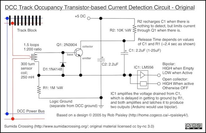
Paisley’s Inductive Detector circuit for use with microprocessor
Parts and ratings:
- coil: originally 300 turn, ~200mH coil, no longer available (see note)
- Q1: 2N3904, NPN, Ic=200 mA, hfe = gain = <100 (typical)
- D1: 1N4148; If = 200 mA max, Vf = 1V @ 100 mA, 0.72V @ 5 mA
Paisley’s circuit originally used a Coilcraft J9119-A (specifications unknown) for the current-sensing coil, now long discontinued. This was replaced by the Vitec 57P1822 (1:350, 73 mH) or alternatively the 57P1820 (1:300, 180mH). He also mentions use of the AS-103 (1:300, 250 mH) as being available in Europe. Coilcraft no longer makes a 300-turn sensor, but its specifications for smaller ones are in line with other manufacturers, so assuming the original was 300 turns, it’s likely to have had inductance around 180 - 250 mH (the 1822 above is rather low in inductance, but there are current equivalents, such as the Triad CST206-3A, Digikey 237-1100-ND, or Pulse PE-51719, Digikey 553-2019-ND, with 300 turns and inductances of 130 and 80 mH respectively).
Note: the two Vitec coils are still available from Surplus Sales of Nebraska (as of October 2013), but both appear to have been discontinued by the manufacturer (I can’t even find a data sheet that lists the 1822 anymore, and the last datasheet describing the 1820 is dated 2007). Neither is available from any of the usual big electronics retailers, which suggests that remaining inventory is low and these aren’t good parts to plan on using (although they’re still available if you only need a few).
For simulation purposes, I’ll assume a 350-turn coil with 73 mH inductance, but I’ll also take a look at the Pulse coil (1:300, 80 mH), as that seems like the best current replacement and compare with a 200 mH coil just in case that was what the original used.
Sensitivity of this detector is claimed to be ~1 mA with 1.5 loops of the feeder through the coil (a 1:233 ratio with the 1822 coil). He also notes that sensitivity is improved with a tight winding of the feeder around the coil, as opposed to just passing the wire through the hole as shown on the datasheets.
And here’s an example of Müller’s circuit, stripped of all non-essentials and showing what would be needed for use with an Arduino digital pin in INPUT mode:
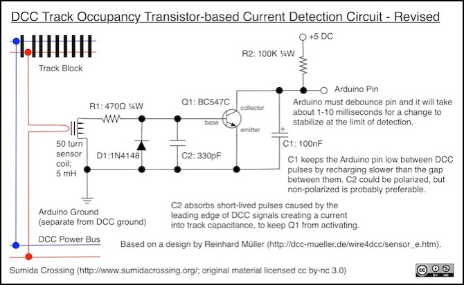
Müller’s Inductive Detector circuit for use with microprocessor
Parts and ratings:
- coil: Nuvotem Talema AS-100 (Digikey TE2301-ND, $3.08 each in qty. 10+); 50 turns, 6 mH @ 10 kHz, 50 ohm resistance
- Q1: BC547C; NPN, Ic = 100 mA, hfe = gain = 270+ (600 typ.)
- D1: 1N4148; If = 200 mA max, Vf = 1V @ 100 mA, 0.72V @ 5 mA
Both the AS-100 coil used by Müller, and an alternate (PE-51686NL, 50 turns, 5 mH) he listed are available from Digikey in updated lead-free designs compatible with the European ROHS regulations, which means they’re relatively new and not likely to be obsoleted any time soon, or the manufacturers wouldn’t have invested in updating to meet ROHS specs; they just would have discontinued them. The other components are commonplace. Müller’s circuit is still a viable one to build as of 2013.
Sensitivity of this circuit is said to be ~1.5 mA of track current.
Sensitivity and Real-world Use
How sensitive does a detector need to be? It depends on what you want to do with the information, and in part on what kind of trains you’re running.
On a DCC layout with track voltage of 10 V DCC (a “worst case” scenario), an axle with a 10 KOhm resistor will draw a current of 1 mA. If you want to detect one car, and only put resistors on one axle per car, that’s your limit. Unless you’re using this with hidden storage tracks, detecting a single car probably isn’t the best criteria. And if it is, you could add resistors that are smaller (a 5 KOhm resistor will draw two milliamps @ 10 V DCC) or put more axles of them on cars that are likely to be left parked alone.
With freight trains, assuming they’re moving forwards, the locomotive will hit the detector first, and it’s drawing tens of mA. Just about anything will detect that. However if you’re switching and back into a grade crossing, you might want to detect that first car (or you could just load up a caboose with more resistors, or smaller ones). Two axles equipped that way will draw 4 mA. In that case, extreme sensitivity probably isn’t needed.
My case is passenger EMUs. These will be lit, but the motor car will be in the middle of the train. I’ve seen lighting draw as little as 3 mA (5 mA+ is more likely), but my cab cars will actually have both interior lighting and a cab decoder with a head/tail-light LED. I need to measure this, but I expect my power draw for cab cars will be close to 10 mA. So I’m not concerned with extreme sensitivity either.
If you really need to, you can make these detectors more sensitive by winding the feeder around the coil more times (although too much of that is likely a bad idea, at least with some of them). You can also make them less sensitive (see the websites for the two authors for discussion of that topic).
Detection time is also a factor here. As currents go down, the circuits take longer to detect a block going occupied (a block going clear is not dependent on current levels). How much the delay matters will depend on the layout. A 40 mph (64 kph) freight is moving a lot slower than a 200 mph (320 kph) bullet train. In 10 milliseconds, an N-scale freight will move 1 mm, while the bullet train will move 6 mm (1/4”). At 100 msec, the freight will have gone 12 mm (1/2”), while the bullet train will have moved 60 mm (2 1/3”). Extend this out to a half-second, and the freight has moved 60 mm (2 1/3”) while the bullet train has moved 296 mm (11 2/3”).
There are certainly situations where waiting a second or more to detect a train is reasonable. But I’ll draw an arbitrary line at a half-second for determining the limit of a detector’s sensitivity.
Comparing the Circuits
It’s instructive to look at the two circuits, and compare how they work. Both use a coil to sense current in a track feeder, and both produce an output that’s either HIGH (close to +5V) or LOW (close to Ground). And both use a capacitor to keep the output stable when there’s nothing to detect, and a transistor as a switch to drain that capacitor when there is. There are significant differences between them in how they go about doing this, and what the end result looks like.
Note: at present my comments on the performance of these circuits is all based on circuit simulations. At some point I’ll probably build a couple of the more interesting solutions, and see what they look like in the real world, but that’s likely some time in the future.
Paisley’s circuit is using R1 to keep the emitter side of the transistor floating above ground. Any voltage released from C1 through Q1 will build up at the input of the 556 integrated circuit, and very, very, slowly drain away through R1. As long as there’s a continuous supply of current into C1, and hence Q1, the input to the IC will remain close to +5V while there is current in the track. Once it goes away, C1 quickly recharges, but the input to the IC slowly drains. The IC very simply takes the input voltage, and above a certain level sets its bipolar input HIGH, indicating that a current flow has been detected (there’s a second output, but it’s less useful for this kind of microprocessor-based sensing). A microprocessor, such as an Arduino, can connect to either of those outputs (or you could just wire up one and ignore the other). C2 in this diagram is simply acting as a filter on the power supply, so that an poorer source of voltage can be used. In fact, per Paisley, this circuit is very tolerant of input voltage, and anything from +5 to +12V can be used.
The circuit is admirably simple: ignoring the filter capacitor, it requires only seven components: coil, diode, transistor, capacitor, two resistors and a LM556. And both R1 and the LM556 can be shared with two detectors, making the component count per detector six.
Müller’s circuit is even more streamlined. In its most basic form: coil, diode, transistor, capacitor and two resistors; the integrated circuit is eliminated. As Müller noted, the improved sensitivity will likely require the addition of C2, but it’s still a simpler circuit. The differences in cost, however, are negligible.
Müller’s circuit operates slightly differently. In it, the state of C1 is sensed directly, and it will be HIGH when no current is flowing in the block. When current flows, Q1 activates and drains C1, but in this case it’s drained straight to ground. Once the voltage in C1 drops below about 2.6V, an Arduino (or similar device) will treat that as a LOW reading. When current stops flowing, C1 recharges and the Arduino will see HIGH once voltage goes above about 4 Volts.
Circuit Simulation
To understand how these circuits work, I needed to simulate them. As I’ve mentioned before, I’m not an electrical engineer, so any of the following could be wrong. My track record on getting these things right is mixed at best, and I don’t have much experience with transistor-based circuits. Use at your own risk. That said, I think I understand what’s going on here.
To simulate these circuits, I needed to build models that would work with a simulator. This is a bit harder than it sounds, because the simulators available to me don’t have a built-in model for a current-sensing coil (I also had problems finding transistor models for the BC547 series, but eventually located those). I made one using a normal transformer with the appropriate turn ratio, but I’m not sure it’s 100% correct (it does seem to produce approximately correct behavior, so I think it’s close). Any errors likely affect each model equally.
To define the transformer, you have to use the inductance of the coil. The SPICE model requires this for both the primary (track feeder) and secondary (coil), but the data sheet only gives the number for the coil. The number for the primary is calculated from the secondary, based on the number of turns of the track feeder, using an inverse-square rule. Here’s the formula, where Ls comes from the datasheet (in millihenrys) and Np/Ns is the ratio of the number of turns of feeder to the number of turns in the coil:
Lp = Ls x (Np / Ns)^2
So, for 1.5 turns of primary into a 300-turn 80 mH coil, you get:
Lp = 80 x (1.5 / 300)^2 = 80 x 0.005^2 = 80 x 0.000025 = 0.002
And thus you set up the transformer with 80 mH in the secondary, and 0.002 mH in the primary.
Note: by definition, simulations are not exact. Models of semiconductors aren’t the same as real ones, and real-world variations between components that are rated identically can be significant at the limits of circuit behavior. While most of what the models are telling me is likely correct, trying to gauge minimum-current sensitivity is quite risky. The fact that my “minimum current” numbers are higher than those of the original authors likely reflects limitations of the model. However, if my model says detector A is 10% more sensitive than detector B, that’s likely true, even if 10% of what may be subject to dispute.
All circuit simulations mentioned here were done in NGSpice 25, using Volta (for OSX) as a graphical front-end to draw the circuits and plot the results. SPICE models were collected from online sources for the specific diode and transistors, but generic models for capacitors, resistors, and coils were used (the coil model was a generic transformer that had parameters set to match the coil’s inductance characteristics; this is probably the weakest portion of the model at present).
Note: all of the simulations of Paisley’s circuit use his recommended 1.5 turns of the track feeder (looping it twice through the hole and then back the way it came, so it can be made snug against the coil). Müller’s description, and a photograph on his site suggest that normal use is to pass the wire through the coil, so I’ve used 1 turn (which is what “go through the hole” is) as the standard configuration for his sensors. He does note that accuracy can be improved with multiple loops, but do did Paisley.
Worst-case Current Performance
Assuming these detectors are used with a 5 Amp DCC supply, the worst case for component tolerances comes when a short happens, sending the full 5 Amps through the track feeder. Obviously, systems can be designed with block-level circuit breakers to limit peak current more (and, alternatively, some people use 8 Amp boosters). But for a reasonably-flexible design, 5 Amps is a good target. It’s also what I’m using today on my layout, although I’m likely moving to a 3A/block approach based on block-level circuit breakers.
Paisley, 1:233 ratio (1.5 turns into 350-turn, 73 mH coil):
This is the Vitec 1822 coil specified as the replacement for the long-unavailable original coil. Unsurprisingly, the detector catches this level of current very quickly, within the first DCC pulse (about 22 microseconds from the start). Voltage applied to the base of Q1 is 1.2V at most, well within safe bounds. Current at the base of Q1 peaks at about 42 mA, and current through the collector-emitter junction (Ice) peaks at 428 mA. This is above the 200 mA limit of the transistor, but only for about 25 microseconds. Once C1 has drained, It won’t recur.
Note: this is for C1 with 2.2 uF. Raising this value will extend the duration of this value, but doesn’t raise the actual current. That’s in line with the transistor characteristics, which have reduced gain as current rises. A 10x gain at currents exceeding 100mA is not unreasonable.
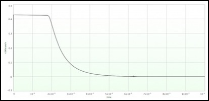
Ice (collector-emitter) current in Amps over first 100 usec after pulse starts (5A feeder current)
Paisley, 1:200 ratio (1.5 turns into 300-turn, 80 mH coil):
Using the best available replacement for the original coil, the Pulse PE-51719, doesn’t noticeably change the detection time for a maximum current pulse. Current into the base rises slightly, to about 50 mA, and Ice climbs slightly to 462 mA, but that’s essentially identical to the original coil for all intents and purposes. The pulse is slightly shorter as well, falling under 200 mA in 23 microseconds.
Paisley, 1:200 ratio (1.5 turns into 300-turn, 130 mH coil):
Because the inductance seemed to play a role in the sensitivity, I decided to look at the behavior of the Triad coil as well. If this has problems, the Vitec 1820 is going to be even worse, making that a poor choice as well. Peak current into the base is now 50 mA and Ice peaks at 463 mA, essentially identical to the Pulse coil. Pulse duration is 25 microseconds.
Müller, 1:50 ratio (1 turn into 50-turn, 5 mH coil):
In the worst case, current into the base spikes to 190 mA, but only remains above 100 mA for about 12 microseconds. Ice peaks at 117 mA, but only for 13 microseconds. This completely drains C1, so it doesn’t happen again on later DCC cycles. I’m not aware of a current limit at the base (Müller states that it’s 500 mA, but that’s not on any data sheet). As with Paisley’s circuit, Ice is exceeding the transistors nominal limit, but similarly only for a very brief time.
Detection time is remarkably fast: just 5 microseconds.
One of the things that concerns me about Müller’s circuit is that the use of a 1:50 coil is producing higher currents in the transistor base, and he’s used a transistor with a lower rating for collector-emitter current and higher gain. I don’t know if that’s a problem, and it doesn’t appear to cause too-high of an Ice current. But it seems like an undesirable feature.
The effect of the much smaller C1 is easily seen in the graph below: the capacitor drains very quickly, so the high current is not sustained (the +/- axis is reversed from the one above because I was sloppy inserting the measurement point in the circuit).
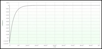
Ice (collector-emitter) current in Amps over first 100 usec after pulse starts (5A feeder current)
Sensitivity
The other extreme is how low a current in the feeder the detector will detect. This is limited by the reduction provided by the coil and the characteristics of the transformer. There’s an interrelated question of how quickly it will detect the current, since detection depends on draining C1, and that takes time. As sensed current drops, the transistor is turned on for shorter intervals each pulse, and the rate of drain goes down quickly. At some point it will be balanced by the recharge rate through the pullup resistor, and that likely sets ti extreme limit of detection. But for practical purposes, I’m going to draw the line a 1/2 second, mostly because longer takes too long to simulate, but also because I think that’s long enough to wait to know that a block has gone occupied.
Note: the time for a block to go clear is different, as it mainly depends on R1 (pulldown) and C2 size in the Paisley circuit and R2 (pullup) and C2 size in the Müller circuit, and doesn’t depend at all on the current being sensed.
Paisley, 1:233 ratio (1.5 turns into 350-turn, 73mH coil):
This circuit has a very predictable behavior: as currents get lower, detection time increases. If there’s limit, it likely lies beyond any reasonable detection time. At 10mA, detection takes about 23 milliseconds. At 5 mA it takes 85 milliseconds. At 3 mA detection time is up to 250 microseconds (a full quarter-second). At 1.5 mA, detection time is 480 microseconds, or essentially a half a second. I’ll draw the line there. It’s not quite the 1 mA of the author’s definition (that likely comes around 3/4 of a second). But it’s still quite good. And, as noted, simulations aren’t going to be exact, particularly at the limits of circuit behavior like this.
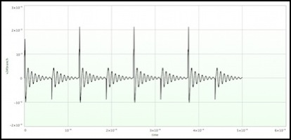
Incidentally, this is what the currents look like from the coil into the base of the transistor, and from collector to emitter (draining C1) during the first four DCC pulses after the block goes occupied (i.e., the first half millisecond). Each of the Ice spikes lasts only about 1 microsecond.
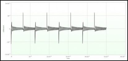
Base current (peak 11 microamps) (1.5 mA feeder current)
Note: the downward spikes are the ones triggering the transistor, a quirk of how I set up the simulation.
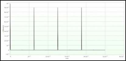
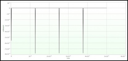
Collector-emitter current (peak 1 mA) (1.5 mA feeder current)
Paisley, 1:200 ratio (1.5 turns into 300-turn, 80 mH coil):
Sensitivity is reduced slightly with the new coil, translating into longer detection times. A 1.5mA track current now takes longer than a half-second to detect (perhaps 2/3), and a 2mA current takes about 425 milliseconds. That’s interesting, as the lower ratio should make the coil more sensitive, not less. The higher inductance is probably playing a role here, as it will choke off the base current pulses faster, lowering the rate at which C1 drains.
Paisley, 1:200 ratio (1.5 turns into 300-turn, 130 mH coil):
Detection time for a 2 mA current does indeed rise slightly, but only to 247 milliseconds. So increasing the mH does have a sensitivity effect, but not a major one.
Paisley, 1:200 ratio (1.5 turns into 300-turn, 250 mH coil):
Just to be complete, I re-ran this analysis for the A-103 coil, to see how a significantly larger mH rating would affect operation. Surprisingly, this improved detection time for 2 mA track current to about 80 milliseconds.
What’s happening here, as you can see below, is that the base pulses are being extended, causing the Ice current to flow for a longer period, and thus draining C1 faster.
Note: the upward spike is the current in the reverse direction before the diode acts to bypass the transistor. It remains short because the diode’s response time doesn’t change, or perhaps because it’s drained the limited charge in the transistor’s base and there’s no more current to flow.
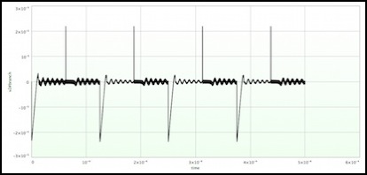
Base current (peak 25 microamps) (1.5 mA feeder current)
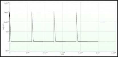
Collector-emitter current (peak 1 mA) (2 mA feeder current)
Müller, 1:50 ratio (1 turn into 50-turn, 5 mH coil):
At 10 mA this circuit takes just 250 microseconds to detect current in the feeder. But as the current drops, this becomes significantly longer. Detection time for 5 mA is 16 milliseconds.
One interesting thing about this circuit is that is has a very solid cut-off of the detection. Once current drops below a threshold, C1 recharges faster than it can drain, and the circuit never falls to a point allowing reliable detection. In my simulation, this happens immediately below 5 mA (4.95 mA fails to work).
Lower the track current below that, and Müller’s circuit stops detecting the change (C1 never gets pulled below 4V, because it’s recharging too fast even with just a 100K pullup; put another way, it’s not draining fast enough. Surprisingly, Paisely’s circuit works at lower currents; it just takes longer and longer to detect things. At 4.3 mA, detection time is 95 milliseconds. At 4 mA it’s about 110 milliseconds. At 3 mA it’s around 180 milliseconds. At 2 mA it’s approaching half a second, and that’s probably a good place to call “done”.
Base current (peak 25 microamps) (5 mA feeder current)
Collector-emitter current (peak 7.8 mA) (5 mA feeder current)
Reset Time
The time it takes the detector to go clear depends on the time it takes the circuit to return to its original state one current is no longer flowing in the feeder and the transistor has turned off. In Paisley’s circuit, this is the time it takes the charge (from C1) at the input of the 556 to drain away through the pulldown resistor (R1). In Müller’s circuit, this is the time it takes C1 to recharge from the pullup resistor (R2).
Both of these are simply defined by the time constant of the RC circuit. C1 needs to recharge to about 80% of full, and the time constant defines how long it will take to recharge to 72% (from zero). But the capacitor may not quite get to zero anyway, so the time constant is a fairly good approximation of the actual time. In practice, it might be slightly longer.
The time constant for Paisley’s circuit is 2.2 seconds (with C1 set to 2.2uF). This can be reduced by reducing the size of C1 (he suggests a lower limit of 1uF) or reducing the size of R1 (but too low may affect sensitivity).
The time constant for Müller’s circuit is much smaller, just 10 milliseconds. This is because of the much smaller value of C1 (and the smaller value of R2 relative to Paisely’s R1). This would be even faster if the internal pullup resistor were used (which varies from ~20 to ~40 kOhm, so times would be about 2 - 4 msec).
Summary
What this all says is that as specified, Paisley’s circuit is more sensitive than Müller’s, although that may in part be due to his addition of the capacitor to prevent false detection of track capacitance-induced currents. Paisley’s circuit is more efficient, tapping off just 0.5% of feeder power compared to Müller’s 2%, but realistically the difference doesn’t matter. Aside from that, Müller’s circuit reacts faster to blocks going both occupied and clear, and has slightly fewer solder joints if you have to hand-build a lot of them.
In a dead short, both of them exceed their transistor’s “safe” level of collector-emitter current, but only briefly. It’s likely that this can be addressed with a simple current-limiting resistor between C1 and Q1, although that may have implications for the circuit’s sensitivity.
I’m not done with my investigation, but I’m probably ready to put it on the back burner and think about what I’ve seen so far. And maybe order some parts to try building a couple and seeing how they actually work. I’ve also played around with simulating some variations on both circuits, to see if their weaknesses can be addressed. This led to some unexpected behavior that I’m still working to understand. I’ll likely add to this page, or add a new page, in the future to discuss that work. But for the moment I’m going to stop here with this analysis of the original circuits.
