Update (3/29/13): The “percent of maximum” numbers are all wrong. I’m never going to get this right. I need to go back and recalculate those, but that’s not happened yet. When it does, I’ll correct this post (and maybe make another one).

===

I really thought I was going to be done with PWM and back to working on decoders this week. But, as is now noted on the last post, I got it wrong. As I mentioned then: “I’m not an electrical engineer. I think I know what I’m talking about, and my conclusions appear to line up with observed reality. But I could have fallen down the rabbit hole and just not noticed. Take it all with due caution and a grain of salt.” Yep, down the rabbit hole I went.

So, as Bullwinkle used to say, “this time for sure!”. Well, sort of. I’ve fixed my problems, but my model isn’t an exact one. For the details of that, and what conclusions I can draw from what I have, read on.

This post of necessity is getting a bit more technical than I’d like. But I don’t think the results can really be understood without some background. I promise, this is the last one on the topic for a while, and I’m going to go back to writing about decoder testing, or maybe layout carpentry, next time.

Just to recap: I’m talking about how DC Permanent Magnet brushed motors used in N-scale model trains operate when driven by Pulse-Wave Modulation (PWM) voltages from a Digital Command Control (DCC) decoder. This is applicable to larger scales, of course, although the specific examples I’m using are drawn from my collection of Japanese-prototype N-scale trains, and the motors in those do have some differences from others.

The problem with my model last time lay in misunderstanding how exponential decay worked to maintain current through the windings, and with two really dumb errors involving the formula. First, I modeled decay as a slow-onset, fast-drop curve, and that’s just not how it works. Rather it’s a “fast drop with a long tail to asymptotic minimum” curve. Second, my decay formula assumed it was starting from the stall current, which made the curve too steep when it was actually starting at a lesser current (because the pulse was too short for current to rise all the way to the stall current). Finally, I messed up converting the growth formula (which I got right) to my spreadsheet, so it produced the wrong shape curve.

In short, I got nearly every bit wrong. What’s worse is that I misread several documents I found online as confirming my interpretation, a classic case of seeing what you want to see.

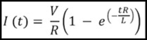
If you’re curious, here are the two formulas involved:

Rising current as a function of time:


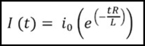
Falling current as a function of time:


where:
I = current in Amps
t = time in seconds
V = maximum voltage of the square wave
R = resistance of the motor in ohms
L = inductance of the motor in Henries
i₀ = current at the start of the decline (maximum current from the prior pulse)
and e is a number roughly equal to 2.718, used for natural logarithms.

Don pointed out that a simulated circuit didn’t work the way my model said it should. And that led me to more reading, and this time I found several documents hat clearly matched Don’s (including one with a scope trace). Then I went through the spreadsheet when it still didn’t look right, and found the additional errors.

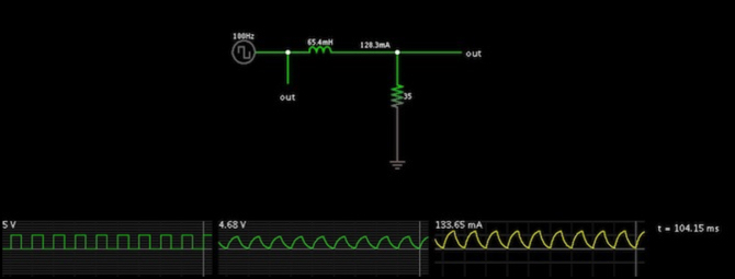
Here’s a snapshot of Don’s simulation of a RL circuit (resistor plus inductor) driven by a square wave (frequency, resistance and inductance chosen to clearly show the waveforms) with a 50% duty cycle (in the graph below, the yellow trace shows current through the circuit). This circuit model was made by Don using a Java-based analog circuit simulator from falstad.com, which is a very handy tool for simulating circuits.



So, back to my model I went.

Here’s an example from the old (incorrect) model:


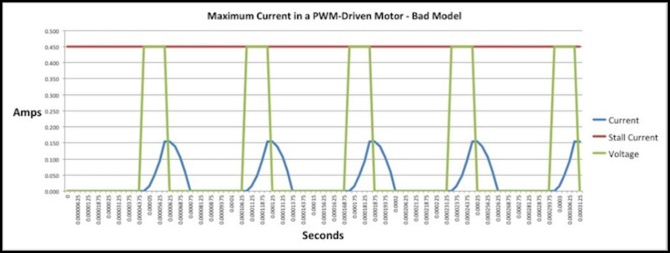
Bad Model, Don’s Circuit



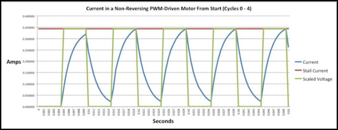
New Model, Don’s Circuit

Looks more correct now, doesn’t it?

What’s happening here is that the fast rise gets the current up higher, and the slower decay curve leaves the current just barely non-zero when the next pulse arrives. My graph is stretched a bit more vertically than the simulators, but leaving that aside they’re nearly identical. The simulator shows a maximum current of 133.65 mA, and my graph is peaking at 133.02 mA, less than a half-percent difference.

I also compared my E231’s numbers for both the circuit simulator and my spreadsheet, and allowing for the differences in presentation they were pretty close (some of the current numbers were off by a few percent, but nothing substantial, and this probably represents rounding error somewhere).

Now that I have a valid model, let’s revisit what this tells me about model train motors and DCC. But first, lets go over motor behavior a bit, and let me explain why this model isn’t quite correct. I still think it’s useful, but it’s ignoring a few important details (as is the circuit simulator).

Motor Design

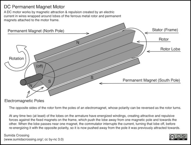
A DC motor is formed of coils of wire wound around lobes of soft iron (or similar metal) connected to a central shaft. These coils (windings) are connected to a power source via a commutator, which reverses their polarity every half-rotation. When a current flows through a winding, it becomes an electromagnet. The frame of the motor has a fixed permanent magnet, with “north” on one side, and “south” on the other. The electromagnet is attracted to one side, and repelled from the other, and as it rotates past the pole and the current reverses, it becomes repelled by the one it was just attracted to. This attraction/repulsion is the force that drives the motor, and is the way it converts electric current to power.

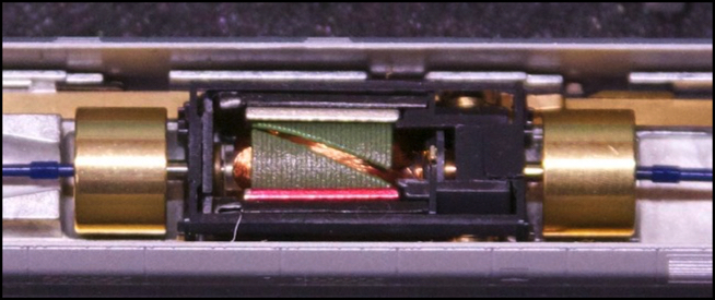
If you look at the photo at the top of the page, the copper-colored wire are the windings, the grayish angled chunks of metal are the rotor lobes (they’re made of stamped metal arranged in layers because it’s a cheap and simple way to make them) and the red and silver bars at top and bottom are the visible poles of the permanent magnet. Hidden inside the black box on the right side are the brushes and commutator, and the motor shaft itself can be seen running from each end of the windings out to the flywheels. The flywheels themselves aren’t part of the motor, any more than the gearbox connecting the drive shaft to the wheels is. They just help by storing momentum if power to the motor is briefly interrupted by dirty track or some other problem.



The basic facts of a DC motor are that voltage produces current, current creates a magnetic field, and magnetic attraction/repulsion rotates the motor and pushes against any load that tries to keep the motor shaft from turning. But it’s not quite as simple as saying “voltage ‘V’ produces speed ’S’”, even though that’s how DC throttles appear to work, and how DCC decoders are programmed.

Current does produce the force of the motor used to overcome torque, so the current is very important. And voltage produces a current, but it’s not as simple as the basic DC Ohm’s Law of I=V/R, although that equation is at the heart of it.

Electrically, a DC Motor can be thought of as a resistor in series with an inductor. The current through the resistor would normally be governed by Ohm’s Law. And, in fact, if the motor isn’t turning, it is. This is the “stall current”, and if you know the resistance of the motor windings and the voltage applied, you can derive the stall current. In practice, I couldn’t measure the resistance accurately with my multimeter, so I had to figure it out from the stall current (which also works).

The presence of the inductor means that current doesn’t immediately rise to the stall current when the voltage is applied, and that’s what I’m modeling today for DCC. But the current it will eventually rise to is actually less than the stall current in a real motor, on DC or DCC, for the following reason.

If the inductor is rotating through a fixed magnetic field (i.e., if the motor is turning rather than stalled), there is an additional reverse voltage created in the inductor that opposes the driving voltage (the resistor is also rotating, but that doesn't change its properties). The effect of this is to reduce the voltage flowing through the circuit since the contrary voltage is subtracted from the driving voltage. The faster the motor turns, the more reverse current is generated by the magnetic field, and the lower the effective voltage.

A fancy name for voltage is “Electromotive Force”, or EMF. This reverse voltage, if you hadn’t guessed already, is the back-EMF (BEMF), although the more common name for it is “Counter EMF” (CEMF). Since DCC decoders often use “BEMF” as shorthand for “BEMF-based duty-cycle stretching compensation”, I’m going to use “CEMF” to describe the actual counter-voltage and “BEMF” for the decoder feature, and I’ll abbreviate the driving voltage as “V” and the counter voltage as “C” for clarity’s sake.



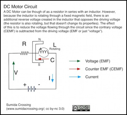
The resulting current “I” through the circuit is I=(V - C)/R. Since C depends on the speed of rotation, a balance is struck when I is enough to overcome the load on the motor. For this reason, current through a running motor will always be less than the stall current. If the load is light, it will be a lot less, even at high speeds. If the load is heavy, it will approach the stall current as the motor slows down and the voltage is increased to full throttle.

For my model of motor operation, I’ve ignored this counter-voltage and assumed that only the driving voltage applies. Thus the current through my model will be equal to the stall current at full voltage. This is exactly how a simple resistor-inductor model of a motor works, and so this is how the simulator mentioned at the beginning of this post works. And thus as noted above, it’s why both aren’t great models for a real motor, except as a way to define the maximum limit.

Now as the load on the motor increases, the differences between the real behavior of the current and my model of it become less, because most of the driving voltage is going to overcoming the drag of the load on the motor, and less is going to make the motor spin. This means my model is more accurate for a motor that’s barely overcoming the load on it. In the real world, this would be as if you had to turn the throttle all the way up, and the train would barely move.

So, in the rest of this post, when I talk about current and DCC duty cycle, understand that the real current is going to be less for a typical train than my 100% number once the motor gets up to speed. But when it’s starting up, most of the voltage is producing current to make torque to get the train moving, and the motor isn’t rotating very quickly, so there’s little counter voltage. So my model is closest to accurate when a train is accelerating.

And so, when I talk about “percentage of maximum impulse” down below, think of this as a relative measure of how well the DCC decoder’s PWM will act to accelerate a stationary train, compared to how well a simple DC throttle would. My model isn’t going to produce a very good picture of what top speed might look like, but it should give a good picture of power available to accelerate a loaded train.

Motor Behavior

There’s another thing to consider here, and at the risk of confusing things I need to bring it up. The minimum “good” PWM frequency has a relationship to maximum motor speed that shouldn’t be ignored. This is completely unrelated to current in the motor, or CEMF. I’m going to talk about both my model of motor current, and the relationship of PWM frequency to possible motor frequency together, because both relate to PWM frequency and possible motor speed. But understand that I’m talking about two different things that relate to PWM frequency, and not (except very indirectly) to each other.

In a typical motor, which can turn at 14,000 RPM at full throttle with no load beyond the friction in the gear train (as does my E231), the typical speed that the motor is turning for a normal speed is probably a few thousand RPM. The exact speed it’s turning is simply a ratio to maximum, so if the train with a given load runs at 180 scale kph at full throttle and the motor turns at 14,000 RPM, then when the train is running at 45 scale kph the motor is turning at 3,500 RPM (25% of 14,000).

That doesn’t necessarily translate to 25% throttle, or to a 25% duty cycle. How those two relate to track speed depends on whether or not BEMF-based compensation (abbreviated BEMF here) or some other compensation is active. Without BEMF, a 25% throttle likely results in a 25% duty cycle (it might not, depending on other things the decoder is doing, like applying a speed curve). But because there’s a non-zero load on the motor, that 25% duty cycle produces less than 25% of maximum train speed. With BEMF, 25% throttle may produce close to 25% speed, but it does so by creating a larger than 25% duty cycle, to provide more power to the motor.

Minimum PWM Frequency

If 14,000 RPM represents top speed, then the motor is turning 233 times per second (14,000/60), or once every 4.3 milliseconds. A half-cycle (the length of time each winding is on) lasts just over 2 milliseconds. To ensure there’s at least one pulse to energize each winding, the pulses must come at a rate of at least once every half cycle, or once every two milliseconds. That’s 500 times a second, or a PWM frequency of 500 Hz (I’m rounding a bit here). It’s probably best to have a couple of pulses per cycle, so I’m going to assume a minimum PWM frequency of 1 kHz (1,000 pulses per second).

The actual number of pulses will vary with speed, but top speed defines the shortest interval. And since PWM frequency doesn’t change with speed, just the length of the pulse within that cycle, this gives us our minimum frequency for a 14,000 RPM motor. A motor with different characteristics, or a train with more or less resistance in its gear train, might turn faster or slower and change the number, and that’s another reason to use a value higher than 500 Hz: to provide a safety margin for faster motors or ones with less friction in the mechanism.

Frequency Example

Let’s assume a scale speed of 45 kph (28 mph), about one-quarter top speed for my E231 (ignoring BEMF for the moment). With wheels of 5.55 mm diameter and a 12:1 gear ratio (which it has), the motor must be turning at about 3,400 RPM, or ~57 rotations per second to produce this speed. This means that the field in the windings is reversing about a 114 times a second, or every 8.8 milliseconds. And if the PWM frequency is 1 kHz, this means that the PWM cycle is repeating (generating a new pulse) once every millisecond, and there are just 8 pulses to establish the field before it reverses.

At very high speed, things are moving more quickly. The loaded top speed is going to be around 180 scale kph (well beyond the maximum I’d need for a commuter train, although I might want a Shinkansen to run this fast). At that speed, the motor is turning 233 times per second, and the length of a pulse (assuming it’s not quite on 100% of the time) about half the time it takes the motor to make a half turn, yielding just more than two pulses.

Duty Cycle, Frequency and Power

An important measure I’m going to use is “Impulse”. This is a measure of energy (the typical value is amp-seconds, meaning the energy contained in a current of one ampere flowing for one second, and an amp-second through a one ohm resistor is a Joule). Mathematically, impulse is the integral of current with respect to time, or in a graphical sense it’s the area under the current curve.

The following diagram shows that 25% duty cycle. The current curve isn’t quite filling the pulse, but the tail after it makes it close. If the area under the green pulse is that maximum possible “Impulse” (energy transferred to the motor), and the area under the blue curve is the actual Impulse, then it’s producing about 76% of the maximum. There’s probably some inefficiency in the wide swings the current is making (this equates to the magnetic field being established and torn down on each pulse, and that has an inefficiency that wastes energy as heat in the windings). But that just means the decoder is drawing more power than the motor needs. The important aspects are the area under the curve (Impulse) as a percent of the maximum, and the number of pulses before the field reverses (more pulses are generally better).

I’m going to summarize those two under each graph for simplicity (and note that pulses per motor cycle is only approximate). Note that longer duty cycles are more efficient because the current has longer to rise and less time to drop with each pulse, and you can clearly see that in the percentage of impulse being produced.


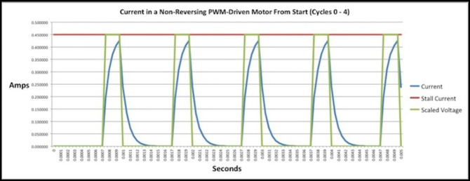
1 kHz PWM, 25% duty cycle, 76% Impulse, 8.7 pulses per cycle (PPC)


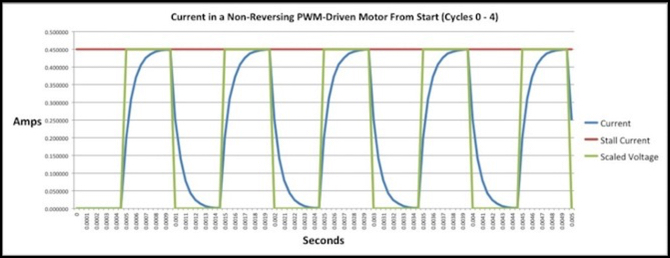
1 kHz PWM, 50% duty cycle, 88% Impulse, 4.4 PPC


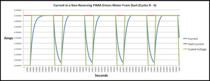
1 kHz PWM, 75% duty cycle, 94% Impulse, 2.9 PPC

With 1 kHz PWM, the motor current easily reaches maximum, and even with fairly long gaps allowing the current to drop down to zero or close to it, the amount of energy being transferred (which ultimately reflects the ability of the motor to do work) is close to that of a DC motor at a similar average voltage (a DC motor would have 100% of the Impulse once it had a chance to rise to full).

Winding Polarity Reversal

There’s something I glossed over here though: every half turn of the motor, the winding reverses polarity (to keep it pulling towards the permanent magnet pole on it is approaching on the present side of the motor). This means that the magnetic field needs to be torn down, so the current can be reversed and a new current established in the other direction. My graphs don’t show this.

However, even though there are only a couple of pulses per half-rotation at high speed, and a handful at low speed, the fact that the current is rising to near full each time means that it doesn’t take long to do that (at worst perhaps one pulse at low speeds, much less at high). The small number of full-current pulses per cycle does point to a likely inefficiency here that I’m not capturing in my “percent of impulse” numbers. And more pulses per cycle, if they rise to maximum, would be preferable for reducing this inefficiency.

At higher frequencies, even though it takes longer to reverse the field (in terms of pulses) there are many more pulses per cycle of the motor. In the end, higher frequencies are probably more efficient in this area overall, but I haven’t worked out the details to be sure.

Faster PWM Frequencies

How does higher-frequency PWM affect Impulse efficiency?

Doubling the frequency makes the pulses (and the gaps) half as long, and the short pulses don’t allow time for the current to rise to full level, which equates to a lower percent of Impulse. However, there are more pulses each cycle, so any initial inefficiency in reversing the field is minimized. And the fact that the gaps between pulses at low speed are long enough for the current to drop to zero on its own means that at most one pulse is lost to reversing the current.

Here’s a summary for several different PWM frequencies at duty cycles of 25%, 50% and 75%. The number of pulses per cycle, meaning the number of pulses before the winding has rotated far enough for the commutator to reverse the current, is estimated based on my E231 assuming a 25% duty cycle equates to 25% speed (so it’s not quite exact, particularly at lower speeds). Efficiency is measured as the impulse per PWM pulse (as a percent of the maximum) after five pulses, to allow current to rise. Where two numbers are given, it’s because it continued rising past this point, and the second reflects roughly the long-term maximum.



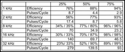
And just to remind you, the percent of maximum impulse is relating the power in the motor relative to the power in a DC motor with the same average voltage ignoring counter-EMF. So it’s a measure of how well the DCC decoder will accelerate a train as compared to a DC throttle.

There’s a clear take-away here: at low duty cycles, high-frequency PWM isn’t very efficient. This is because the pulses are too short, and the gaps too long, for the current to establish itself at more than a small fraction of the stall current. This isn’t necessarily bad, if you have BEMF or some other compensation mechanism. It just means that the duty cycles for low speed will need to be stretched to give enough power to pull a load. It might ultimately represent less total power available, but probably not.

And the reason is that at high duty cycles the pulses last long enough to get the efficiency up. The difference between 8 kHz and 32 kHz isn’t really that much at 75% duty cycle (96% vs 99%), so it’s not really saying that there’s an advantage to the higher frequencies. But there’s no problem either.

Now what this does point out, quite strongly, is than an unmodified duty cycle is going to have less pulling power at higher frequencies, and so you’d either need to turn the throttle up higher to move a heavy train, or have a speed table that maps lower throttles to higher percentages of average voltage (remember that decoders work with fractions of full voltage). Or you’d need something like BEMF to stretch the duty cycle to get the necessary speed.

In short, with supersonic decoders, you REALLY need BEMF or some other adaptive compensation mechanism at low speeds to accelerate a train or help it climb grades, and as the PWM frequency is raised you need it at higher speeds also, but you can ultimately have it cut out somewhere between 50% and 75%.

And that’s basically my take-away: BEMF is most important at “low” speeds, but that low speed can actually be quite high if the PWM frequency is high also. Since most decoders today are “supersonic” and work around 16 kHz, that means that BEMF is needed at up to a significant percentage of the throttle. And since on my commuter trains, top standard speed is 120 kph, or about 67% of maximum, this means I need BEMF over most of my usable voltage range, and I probably won’t use the “BEMF Cutout” CV even on those decoders that offer one.

Hopefully I haven’t totally confused everyone with this post. It’s had a lot more words, and a lot less clarity, than I strive for.

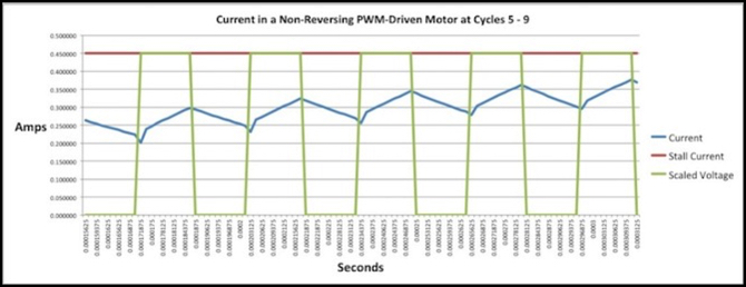
I’ll close with a couple of illustrative graphs out of my model, although I’m not going to show all of the ones that went into making the table up above. I’ve already shown the 1 kHz chart. I’m going to skip the first five pulses when the motor is just starting (numbered 0 to 4 in my model) and show the next five (numbered 5 to 9) when the current has mostly reached the maximum level.

First 8 kHz: the shorter pulses prevent the current from getting up to maximum, which is why the impulse at lower duty cycles is poorer than the 1 kHz PWM. But for longer pulses, the short gaps keep the current from dropping too far, and lift the overall impulse higher.



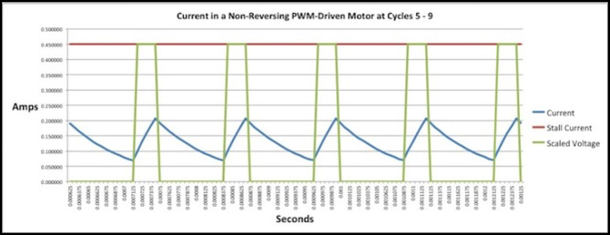
8 kHz PWM, 25% duty cycle, 35% Impulse


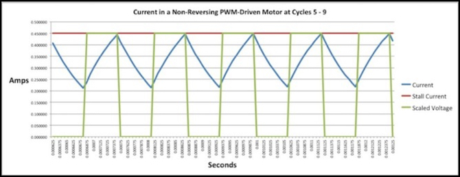
8 kHz PWM, 50% duty cycle, 80% Impulse


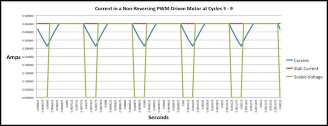
8 kHz PWM, 75% duty cycle, 96% Impulse

At higher frequencies, the charts don’t look substantially different, except that it takes longer to rise to the full value of current (longer in terms of pulses, in actual milliseconds it’s probably about that same). And at higher frequencies the difference between maximum and minimum is less. I’ll close with two charts, showing 16 kHz and 32 kHz PWM, both at 50% duty cycle. In fact, at 32 kHz, even by pulse #10 the current is well short of the level it will eventually reach. But compare these to the 8 kHz 50% duty-cycle chart above, and the differences are obvious.


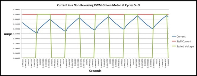
16kHz PWM, 50% duty cycle, 87% Impulse


32kHz PWM, 50% duty cycle, still below maximum Impulse (which will be 90%)

Tags: DCC, Design, PWM